Statistical Learning Theory: Slow and fast learning bounds
Extract from my upcoming thesis - 20/03/20
Statistical learning theory
Summary: This chapter is a short introduction to statistical learning theory, which focuses on the derivation of bounds on the generalization error for the binary classification problem. For that matter, we first present the probabilistic setting associated to binary classification and the associated risks. Then, to bound the excess risk of the empirical minimizer, we introduce a few basic concentration inequalities, followed by strategies to relate the excess risk to the complexity of a proposal class, which enable us to derive generalization bounds that are independent of the distribution of the data. Next, we address the looseness of those bounds with more involved concentration inequalities, which, combined with noise assumptions on the distribution of the data, imply fast, distribution-dependent bounds on the generalization error. Finally, we dwelve into the necessary notions to extend those results for the problems tackled in the thesis, and refer to the specific parts of those that require the tools and results presented here. We refer the reader to (Bousquet, Boucheron, and Lugosi 2004), (Boucheron, Bousquet, and Lugosi 2005) and (Györfi 2002) for more detailed introductions on statistical learning theory.
1 - Introduction
Statistical learning theory is described in (Bousquet, Boucheron, and Lugosi 2004, chap. 1) as a mathematical framework for studying the problem of inference, that is of gaining knowledge about some modeled phenomenon from data. It can be considered as a mathematical tool that justifies the soundness of performing machine learning, i.e. of using data collected in some specific context, e.g. in the past, to make decisions in another context, e.g. in the future. For that to be sensible, one has to make assumptions as to how the data collected - called training data - relates to the testing data, and those assumptions are referred to as inductive bias.
Generally, one collects data that belong to a input space \(\mathcal{X}\), also called feature space, that is often a \(d\)-dimensional Euclidean space, i.e. \(\mathcal{X}= \mathbb{R}^d\). Using that information, one wishes to gain knowledge about some value that belongs to an output space \(\mathcal{Y}\). To study the relationship between the collected features and the output value, those are modeled as a pair of dependent random variables r.v. \((X, Y) \in \mathcal{X}\times\mathcal{Y}\) that follow some unknown joint distribution \(P\) defined on a probability space \((\Omega, \mathcal{A}, \mathbb{P})\). We refer to the two first chapters of (Shorack 2000) for a thorough definition of these mathematical objects. The random variable \(Y\) is referred to as the output r.v., while \(X\) is referred to as the input r.v.. We introduce the distribution of \(X\) as \(F\), called the marginal distribution of \(X\), see (Papoulis 1965 Chapter 6, page 171). Mathematically, statistical learning theory is generally interested in recovering some information about distribution of the output r.v. for any possible value of the input r.v. \(X\), i.e. about the conditional random variable \(Y | X=x\) for any \(x \in A\), with \(A \subset \mathcal{X}\) such that (s.t.) \(\mathbb{P}\{X \in A \}=1\). The distribution \(P\) can be decomposed as \(F \times P_{Y|X}\), with \(P_{Y|X}\) the conditional distribution of \(Y\) given \(X\). It is referred to as the posterior probability of \(Y\), and its existence is justified in (Shorack 2000 Chapter 8, Theorem 5.2).
Many learning problems assume that the output random variable \(Y\) is binary, i.e. \(\mathcal{Y}= \{ -1, +1 \}\), such as binary classification or bipartite ranking. Under that assumption, the posterior probability \(P_{Y|X}\) is summarized by the mapping \(\eta\) with: \[\begin{align} \eta : \; \mathcal{X}&\to [0,1],\\ x & \mapsto \mathbb{P}\{ Y=+1 \mid X=x\},\end{align}\] which is referred to as the regression function or as the Bayes scorer in the bipartite ranking literature. The distribution \(P\) is completely characterized by the pair \((F, \eta)\). Another way to specify \(P\) is to define the proportion of positive instances \(p = \mathbb{P}\{ Y = +1 \}\) and the distribution of the conditional random variables \(X|Y=y\) with for both \(y = +1\) and \(y = -1\) as \(G\) and \(H\), respectively. Then, the two characterizations are related by the relations \(G = \eta F/p\) and \(H = (1-\eta)F/(1-p)\) and \(p = \int \eta(x)dF(x)\). They imply \(F = pG + (1-p)H\) and \(\eta/(1-\eta) = pG/( (1-p)H)\).
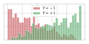
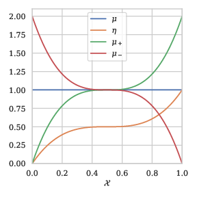
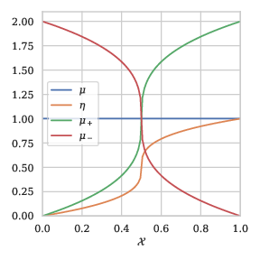
Example 1: To illustrate this section, we provide an example with \(\mathcal{X}= [0,1]\). We introduce a posterior probability \(\eta\), that depends on the parameter \(a \in (0,1)\): \[\begin{align} \eta(x) = \frac{1}{2} + \frac{1}{2} \text{sgn}(2x-1){ \lvert 1-2x\rvert }^{\frac{1-a}{a}}. \end{align}\] See Figure 1 for a representation of the characterizations of \(P\) for \(a=1/2\).
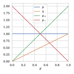
Representation of \(P\)
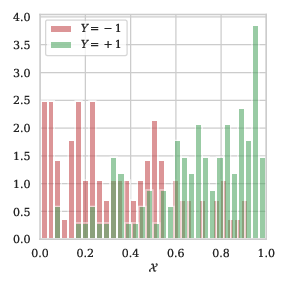
Dist. \(n=200\)
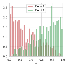
Dist. \(n=1000\)
We now focus on the binary classification problem, and refer to the thesis for a discussion on the extension of those results to other settings. The goal of binary classification is to find a function \(g: \mathcal{X}\to \mathcal{Y}= \{-1, +1\}\) in a class of candidate functions \(\mathcal{G}\) that minimizes the misclassification error \(R(g)\), \[\begin{align} R(g) := \mathbb{P}\{ g(X) \ne Y \}.\end{align}\] The following proposition characterizes the best classifier in the set of all measurable functions.
Proposition 6: The Bayes classifier is defined as the function \(g^*: \mathcal{X}\to \mathcal{Y}\) s.t.: \[\begin{align} \forall x \in \mathcal{X}, \quad g^*(x) := 2\mathbb{I}\{ \eta(x) > 1/2\} - 1. \end{align}\] For any measurable \(g : \mathcal{X}\to \mathcal{Y}\), we have \(R(g^*) \le R(g)\).
Furthermore, we have the following decomposition of the excess risk: \[\begin{align} \label{eq-decomposition-excess-risk}\tag{1} R(g) - R(g^*) = \mathbb{E}[{ \lvert 2\eta(X) - 1 \rvert } \cdot \mathbb{I}\{ g(X) \ne g^*(X) \}]. \end{align}\]
Proof. Note that: \[\begin{align} R(g) = \mathbb{E}[ \mathbb{E}[ \mathbb{I}\{ g(X) \ne Y \} | X ] ] = \mathbb{E}[ \eta(X) + (1-2\eta(X)) \mathbb{I}\{ g(X) = +1 \} ]. \end{align}\] Since: for any \(x \in \mathcal{X}\) and \(g : \mathcal{X}\to \mathcal{Y}\), \[\begin{align} (1-2\eta(x))\left( \mathbb{I}\{g(x) = +1 \} - \mathbb{I}\{ g^*(x) = + 1\} \right) = { \lvert 2\eta(x)-1\rvert } \cdot \mathbb{I}\{ g(x) \ne g^*(x) \}, \end{align}\] we have that \(R(g) \ge R(g^*)\) for any measurable \(g\). □
Note that \(R(g^*) = \mathbb{E}[\min(\eta(X), 1-\eta(X))]\), which means that \(g^*\) has a positive risk unless \(\eta(X) \in \{0, 1\}\) a.s., which means that the Bayes classifier makes classification mistakes unless the classes are separable. A sensible goal when selecting a candidate function in \(\mathcal{G}\) is to find \(g \in \mathcal{G}\) with \(R(g)\) as close as possible to \(R(g^*)\), which is measured by the notion of excess risk, defined as: \[\begin{align} E(g) := R(g) - R(g^*).\end{align}\]
Remark 4: The Bayes classifier of Example 1 is the simple function \(x \mapsto \mathbb{I}\{ x \ge 1/2\}\). In that case, it belongs to the simple proposal class of functions \(\mathcal{G}_{\text{stump}}\) that consists of all of the decision stumps on \([0,1]\), i.e. \(\mathcal{G}_{\text{stump}} = \{ x \mapsto a \cdot \text{sgn}( x - h ) \mid h \in [0,1], a \in \{-1, +1 \} \}\).
Unlike for Remark 4, in most cases, the class \(\mathcal{G}\) is not large enough to contain the Bayes classifier \(g^*\). Then, the gap in performance between any minimizer \(g^\dagger\) of \(R\) in \(\mathcal{G}\), i.e. \(g^\dagger \in {\arg \min}_{g\in\mathcal{G}} \; R(g)\), and \(g^*\) is quantified by the approximation error defined as: \[\begin{align} R(g^\dagger) - R(g^*) > 0.\end{align}\] Controlling the approximation error generally requires an assumption about the smoothness of the target function. One way to introduce this type of assumption is to assume that the regression function \(\eta\) belongs to a Sobolev space, see (Jost 2011 Appendix A.1). While results exist in the case of regression, see e.g. (Smale and Zhou 2011), bounding the approximation error in classification remains an open problem.
Since \(P\) is unknown, we cannot directly measure the risk \(R\). The general idea of statistical learning is to use a notion of empirical risk to approximate \(R\). Introduce a sequence of \(n\) i.i.d. pairs with the same distribution as \((X,Y)\), i.e. \(\mathcal{D}_n = \{(X_i, Y_i)\}_{i=1}^n \overset{\text{i.i.d.}}{\sim} P\), we define the empirical risk \(R_n\), on the data \(\mathcal{D}\) as: \[\begin{align} \label{eq-estimate-empirical-risk}\tag{2} R_n(g) := \frac{1}{n} \sum_{i=1}^n \mathbb{I}\{ g(X_i) \ne Y_i \},\end{align}\] and denote by \(g_n\) the minimizer of \(R_n\) over \(\mathcal{G}\). The precision of the approximation of \(R\) by \(R_n\), and as a result, the choise of \(g_n\), depends on the difference between the empirical distribution and the real distribution, illustrated in Section 3. A quantity of interest is the risk \(R(g_n)\) of the minimizer of the empirical risk, as it quantifies the performance of the classifier learned from data. Observe, that, since \(R_n(g_n) \le R_n(g^\dagger)\) by definition of \(g_n\), we have: \[\begin{align} E(g_n) &\le R(g^\dagger) - R(g^*) + R(g_n) - R_n(g_n) + R_n(g^\dagger) - R(g^\dagger),\\ &\le R(g^\dagger) - R(g^*) + 2 \sup_{g\in\mathcal{G}} { \lvert R_n(g) - R(g)\rvert }. \label{eq-sup_emp_bound}\tag{3}\end{align}\] Eq. (3) shows that one can bound the excess of risk by the approximation error plus the uniform deviation \({ \lVert R_n - R\rVert }_{\mathcal{G}} := \sup_{g\in\mathcal{G}} { \lvert R_n(g) - R(g)\rvert }\) of \(R_n(g) - R(g)\) over \(\mathcal{G}\), which quantifies the generalization error. The bound can be seen as a formalization of the bias-variance tradeoff presented in (Domingos 2012), where the bias term corresponds to the approximation error, while the variance corresponds to the generalization error. When one increase the size of the proposal family \(\mathcal{G}\), the approximation error decreases, while the generalization error increases.
The learning bounds presented throughout the thesis consist in PAC (probably approximately correct)-style bounds, i.e. bounds satisfied for any outcome \(\omega \in A_\delta\) for some \(A_\delta \subset \Omega\) with \(\mathbb{P}\{ A_\delta \} \ge 1 - \delta\), for similar types of uniform deviations over diverse families of functions. All of the bounds concern the generalization error.
Firstly, Section 2 shows how to derive an uniform learning bound, i.e. bounds that do not depend on the distribution of the data, i.e. that hold for the most complicated distributions \(P\) possible, but tend to be quite loose for sensible distributions. Secondly, Section 3 responds to this weakness by deriving tighter bounds under mild assumptions on the data. Finally, Section 4 discusses the extension of such results to the more complicated statistics involved in the thesis and indexes the uses of the tools and results of this chapter in the thesis.
2 - Uniform learning bounds
Most learning bounds are based on the Chernoff bound, which bounds the tail \(\mathbb{P}\{ Z > t\}\) of a r.v. \(Z\) using its moment generating function \(\lambda \mapsto \mathbb{E}[e^{\lambda Z}]\), as shown below.
Proposition 3: (Boucheron, Lugosi, and Massart 2013, sec. 2.1) For any real-valued r.v. \(Z\) and any \(t \in \mathbb{R}\), \[\begin{align} \label{eq-chernoff-bound}\tag{4} \mathbb{P}\left\{ Z > t \right\} \le \inf_{\lambda > 0} \mathbb{E}\left[ e^{\lambda (Z-t)} \right] = \inf_{\lambda > 0} \left( \mathbb{E}\left[ e^{\lambda (Z-\mathbb{E}[Z]) } \right] \cdot e^{\lambda ( \mathbb{E}[Z] - t )} \right), \end{align}\]
Proof. The proof is a simple combination of an increasing transformation with Markov’s inequality. Let \(\lambda > 0\), then \(t \mapsto e^{\lambda t}\) is increasing and the simple bound \(\mathbb{I}\{ x > 1 \} \le x\) holds for \(x \in \mathbb{R}\), hence: \[\begin{align} \label{eq-inter-proof-chernoff}\tag{5} \mathbb{P}\left\{ Z > t \right\} = \mathbb{P}\left\{ e^{\lambda Z} > e^{\lambda t} \right\} = \mathbb{E}\left[ \mathbb{I}\{ e^{\lambda(Z-t)} > 1 \} \right] \le \mathbb{E}\left[ e^{\lambda (Z-t)} \right], \end{align}\] and minimizing the right-hand side of Eq. (5) gives the result. □
By substituting \(Z\) with \({ \lVert R_n - R\rVert }_\mathcal{G}\) in Eq. (4), one sees that controlling the uniform deviation can be achieved by combining two separate results. Specifically, one needs to control \(\mathbb{E}[Z]\), a term that measures the expressivity of the proposal class \(\mathcal{G}\), and a term \(Z-\mathbb{E}[Z]\) a term that measures the robustness of the process of selecting \(g\) from data. For sensible families \(\mathcal{G}\), both of these quantities decrease to zero when \(n\) increases, but with different convergence speeds. The parameter \(\lambda\) is typically selected to balance the speeds of convergence of the two terms.
Section 2.1 presents basic concentration inequalities, that are required to study the terms \(\mathbb{E}[Z]\) and \(Z-\mathbb{E}[Z]\) where \(Z = { \lVert R_n - R\rVert }_\mathcal{G}\). Controlling the convergence of \(\mathbb{E}[Z]\) is based on controlling the complexity of the proposal class of functions \(\mathcal{G}\), which is dealt with in Section 2.2. Finally, Section 2.3 exploits the results of Section 2.2 and the McDiarmid’s inequality presented in Section 2.1 to conclude.
2.1 - Basic concentration inequalities
Three distinct but related formulations exist for any result of Section 2.1. One can write as a bound on the tail \(\mathbb{P}\{Z>t\}\) of a r.v. \(Z\), or a bound on the moment generating function \(t \mapsto \mathbb{E}[e^{tZ}]\) of a r.v. \(Z\), which relates simply to the tail of \(Z\) with Chernoff’s bound, see Proposition 3. One form implies the other, and all theorems can be stated in any of those two forms. Finally, consider a bound on the tail of a r.v. \(Z\) that writes \(\mathbb{P}\{ Z > t \} \le f(t)\), and define \(t_\delta\) as the solution in \(t\) of \(\delta = f(t)\) with some \(\delta > 0\). The bound \(\mathbb{P}\{ Z > t \} \le f(t)\) is then equivalent to a simple inequality of the form \(Z \le t_\delta\), that holds with probability (w.p.) larger than (\(\ge\)) \(1-\delta\). For example, Corollary 3 below is provided in that last formulation.
The most famous concentration inequality is Hoeffding’s inequality (Györfi 2002 Theorem 1.2), which gives a PAC bound on the deviation of the mean of bounded i.i.d. r.v.’s from their expectation of the order \(O(n^{-1/2})\). It stems from a simple bound on the tail \(\mathbb{P}\{ Z > t\}\) of a bounded random variable \(Z\), a property introduced in (Györfi 2002 Lemma 1.2 ) and presented in the lemma below.
Lemma 1: Let \(Z\) be a random variable with \(\mathbb{E}[Z] = 0\) and \(a\le Z \le b\) a.s.. Then for \(t > 0\): \[\begin{align} \mathbb{E}\left[ e^{tZ} \right] \le e^{t^2 (b-a)^2 / 8}. \end{align}\]
Proof. The proof of this lemma is the beginning of the proof of the Hoeffding inequality detailed in (Györfi 2002 Lemma 1.2) and is recalled here for completion. By convexity of the exponential function: \[\begin{align} e^{tz} \le \frac{z-a}{b-a} e^{tb} + \frac{b-z}{b-a} e^{ta} \quad \text{for } a \le z \le b. \end{align}\] Exploiting \(\mathbb{E}[Z] = 0\), with \(p = - a/(b-a)\): \[\begin{align} \mathbb{E}[e^{tZ}] & \le -\frac{a}{b-a} e^{tb} + \frac{b}{b-a} e^{ta},\\ & \le \left( 1 - p + pe^{s(b-a)} \right) e^{-ps(b-a)} = e^{\phi(u)}. \end{align}\] with \(u = s(b-a)\), and \(\phi(u) := -pu + \log(1-p + pe^u)\). The derivative of \(\phi(u)\) is: \[\begin{align} \phi'(u) = -p + \frac{p}{p + (1-p) e^{-u}}, \end{align}\] therefore \(\phi(0) = \phi'(0) = 0\). Moreover, \[\begin{align} \phi''(u) = \frac{p(1-p) e^{-u}}{\left( p + (1-p) e^{-u} \right)^2} \le \frac{1}{4}. \end{align}\] By a Taylor series expansion with remainder, for some \(\theta \in [0,u]\), \[\begin{align} \phi(u) = \phi(0) + u \phi'(0) + \frac{u^2}{2} \phi''(\theta) \le \frac{u^2}{8} = \frac{s^2(b-a)^2}{8}, \end{align}\] which concludes the proof. □
Corollary 3: Let \(Z_1, \dots Z_n\) be \(n\) i.i.d. r.v. s.t. \(a \le Z_1 \le b\). Denote their mean by \(\bar{Z}_n = (1/n)\sum_{i=1}^n Z_i\). Then for any \(\epsilon > 0\), we have w.p. \(\ge\) \(1-\epsilon\), \[\begin{align} \bar{Z}_n - \mathbb{E}[\bar{Z}_n] \le (b-a) \sqrt{\frac{\log(1/\delta)}{2n}}. \end{align}\]
Proof. By Chernoff’s bound, see Proposition 3, we have: \[\begin{align} \label{eq-proof-hoeffding-chernoff}\tag{6} \mathbb{P}\{ \bar{Z}_n - \mathbb{E}[\bar{Z}_n] > t \} \le \inf_{\lambda > 0} e^{-t\lambda} \mathbb{E}\left[ e^{\lambda(\bar{Z}_n- \mathbb{E}[\bar{Z}_n])}\right]. \end{align}\] The independence between the \(Z_i\)’s, see (Shorack 2000 Chapter 8, Theorem 1.1), followed by Lemma 1, implies that: \[\begin{align} \mathbb{E}\left[ e^{\lambda(\bar{Z}_n- \mathbb{E}[\bar{Z}_n])}\right] = \prod_{i=1}^n \mathbb{E}\left[ e^{(\lambda/n) (Z_1 - \mathbb{E}[Z_1])}\right] = e^{ \lambda^2 (b-a)^2 / (8n)}. \end{align}\] Minimizing the r.h.s. of Eq. (6) in \(\lambda\) gives: \[\begin{align} \label{eq-proof-to_invert_hoeffding}\tag{7} \mathbb{P}\{ \bar{Z}_n - \mathbb{E}[\bar{Z}_n] > t \} \le e^{-2t^2 n /(b-a)^2}. \end{align}\] Inverting that bound, i.e. solving in \(t\) such that \(\delta\) is equal to the r.h.s. of Eq. (7) implies the result. □
One can bound the tail of \({ \lvert \bar{Z}_n - \mathbb{E}[\bar{Z}_n]\rvert }\) using the union bound, also referred to as the subadditivity of measures or Boole’s inequality, (Shorack 2000 Chapter 1, Proposition 1.2), between Corollary 3 and its application to the family \(-Z_1, \dots, - Z_n\), which writes: \[\begin{align} \mathbb{P}\{ { \lvert \bar{Z}_n - \mathbb{E}[\bar{Z}_n] \rvert } > t \} \le \mathbb{P}\{ \bar{Z}_n - \mathbb{E}[\bar{Z}_n] > t \} + \mathbb{P}\{ \mathbb{E}[\bar{Z}_n] - \bar{Z}_n > t \} \le 2 e^{-2t^2 n /(b-a)^2}.\end{align}\]
The Hoeffding inequality on its own implies guarantees for finite families of functions \(\mathcal{G}\), as presented in (Bousquet, Boucheron, and Lugosi 2004, sec. 3.4) and shown in the corollary below:
Corollary 1: Assume that \(\mathcal{G}\) is of cardinality \(N\). Then, we have that, for any \(\delta > 0\) and \(n\in\mathbb{N}\), w.p. \(\ge 1-\delta\): \[\begin{align} R(g_n) - R(g^\dagger) &\le \sqrt{ \frac{2}{n} \log \left( \frac{2N}{\delta} \right) }. \end{align}\]
Proof. The union bound implies: \[\begin{align} \mathbb{P}\{ \max_{g\in\mathcal{G}} { \lvert R_n(g) - R(g)\rvert } > t \} & = 1 - \mathbb{P}\{ \cup {g\in\mathcal{G}} { \lvert R_n(g) - R(g)\rvert } \le t \}, \\ & \ge 1 - \sum_{g\in\mathcal{G}} \mathbb{P}\{ { \lvert R_n(g) - R(g)\rvert } \le t \}. \end{align}\] Applying Corollary 3 gives: \[\begin{align} \mathbb{P}\{ \max_{g\in\mathcal{G}} { \lvert R_n(g) - R(g)\rvert } \le t \} & \le \sum_{g\in\mathcal{G}} \mathbb{P}\{ { \lvert R_n(g) - R(g)\rvert } \le t \}, \\ & \le 2N e^{-2t^2 n }, \end{align}\] and inverting the bound gives the result. □
The result presented in Lemma 1 can be used to derive bounds on the expectation of the maximum of a family of random variables, as shown in the following lemma. It is useful when considering minimizers of the empirical risk, to upper-bound the value of \(\mathbb{E}[{ \lVert R_n - R\rVert }_\mathcal{G}]\) presented in Section 1.
Lemma 3: (Györfi 2002 Lemma 1.3) Let \(\sigma > 0\), and assume that \(Z_1, \dots, Z_m\) are real-valued r.v.’s such that for any \(t > 0\) and \(1\le j \le m\), \(\mathbb{E}[e^{t Z_j}] \le e^{t^2 \sigma^2 /2}\), then: \[\begin{align} \mathbb{E}\left[ \max_{j\le m} Z_j \right] \le \sigma \sqrt{\log (2m)}. \end{align}\]
Proof. Jensen’s inequality, which states that that for any integrable r.v. \(Z \in \mathbb{R}\) and any convex function \(\phi: \mathbb{R}\to \mathbb{R}\), we have \(\phi(\mathbb{E}[X]) \le \mathbb{E}[\phi(X)]\), see (Shorack 2000 inequality 4.10 in chapter 3 ), implies that, for any \(t > 0\), \[\begin{align} e^{t\mathbb{E}\left[ \max_{j\le m} Z_j \right]} \le \mathbb{E}\left[ e^{t \max_{j\le m} Z_j } \right] = \mathbb{E}\left[ \max_{j \le m} e^{t Z_j} \right] \le \sum_{j=1}^m \mathbb{E}\left[ e^{t Z_j} \right] \le m e^{t^2 \sigma^2 /2}. \end{align}\] Thus, with \(t = \sqrt{2\log(m) /\sigma^2}\), \[\begin{align} \mathbb{E}\left[ \max_{j\le m} Z_j \right] \le \frac{\log(m)}{t} + \frac{t\sigma^2}{2} = \sigma \sqrt{2\log(m)}, \end{align}\] which concludes the proof. □
One can again bound the tail of \(\max_{j\le m} { \lvert Z_j\rvert }\) by applying the preceding result to a family of \(2m\) elements by considering \(\max(Z_1, -Z_1, \dots, Z_m, -Z_m)\). Now that we have presented inequalities to deal with the term \(\mathbb{E}[{ \lVert R_n - R\rVert }_\mathcal{G}]\), we introduce the one that controls the deviation of \(\mathbb{E}[{ \lVert R_n - R\rVert }_\mathcal{G}]\) from its mean.
Theorem 2: (Györfi 2002 Lemma 1.4 ) Let \(Z_1, \dots, Z_n\) be a collection of \(n\) i.i.d. random variables. Assume that the some function \(g: \text{Im}(Z_1)^n \to \mathbb{R}\) satisfies the bounded difference assumption, i.e.: \[\begin{align} \sup_{ \substack{z_1,\dots,z_n \in \text{Im}(Z_1)\\ z_i' \in \text{Im}(Z_1)} } { \lvert g(z_1, \dots z_n) - g(z_1, \dots, z_i', \dots, z_n) \rvert } \le c_i, \qquad 1\le i \le n, \end{align}\] then, for all \(t > 0\): \[\begin{align} \mathbb{P}\{ g(Z_1, \dots, Z_n) - \mathbb{E}[ g(Z_1, \dots, Z_n) ] > t \} \le \exp \left\{ - \frac{2 t^2}{\sum_{i=1}^n c_i^2} \right\}. \end{align}\]
Proof. For any \(z_i \in \text{Im}(Z_1)\), introduce: \[\begin{align} V_i &= \mathbb{E}\left[ g(Z_1, \dots, Z_n) \mid Z_1, \dots, Z_i \right] - \mathbb{E}\left[ g(Z_1, \dots, Z_n) \mid Z_1, \dots, Z_{i-1} \right],\\ W_i(z_i) &= \mathbb{E}\left[ g(Z_1, \dots, z_i, \dots, Z_n) - g(Z_1, \dots, Z_n) \mid Z_1, \dots, Z_{i-1} \right]. \end{align}\] Note that \(W_i\) is a random function \(\text{Im}(Z_1) \to \mathbb{R}\) that only depends on the \(Z_1,\dots, Z_{i-1}\), hence \(W_i(Z_i) = V_i\). The definition of \(V_i\) gives the following telescopic sum: \[\begin{align} \label{eq-proof-mcdiarmid-decomp}\tag{8} g(Z_1, \dots, Z_n) - \mathbb{E}[ g(Z_1, \dots, Z_n) ] = \sum_{i=1}^n V_i. \end{align}\] Then \(\inf_{z} W_i(z) \le V_i \le \sup_{z} W_i(z)\) and: \[\begin{align} \sup_{z} W_i(z) - \inf_{z} W_i(z) = \sup_{z} \sup_{z'} (W_i(z) - W_i(z')) \le c_i. \end{align}\] For any \(i \in \{1, \dots, n\}\), from Lemma 1 above conditioned upon the \(Z_1, \dots, Z_{i-1}\): we have that, for any \(t > 0\): \[\begin{align} \mathbb{E}\left[ e^{tV_i} \mid Z_1, \dots, Z_{i-1} \right] \le e^{t^2 c_i^2 / 8}. \end{align}\] Finally, \[\begin{align} \mathbb{E}\left[ e^{ t \left( \sum_{i=1}^n V_i \right) } \right] \le \mathbb{E}\left[ e^{t \sum_{i=1}^{n-1} V_i} \mathbb{E}\left[ e^{t V_n} \mid Z_1, \dots, Z_{n-1} \right] \right] \le e^{t^2 \sum_{i=1}^n c_i^2 / 8}, \end{align}\] by repeating the same argument \(n\) times. Minimizing the Chernoff bound implies the result. □
2.2 - The complexity of classes of functions
This section regroups several ways used to control the complexity of a class of proposal functions \(\mathcal{G}\), referred to as capacity measures in (Boucheron, Bousquet, and Lugosi 2005). Those include Rademacher averages, the concept of shatter coefficient and VC dimension, as well as covering numbers. First, we introduce the notion of Rademacher average and relate it to the notion of VC dimension. For an introduction to covering numbers in this context, we refer to (Boucheron, Bousquet, and Lugosi 2005 Section 5.1).
Definition 2: The Rademacher average of \(\mathcal{G}\) is defined as: \[\begin{align} \mathfrak{R}_n(\mathcal{G}) := \mathbb{E}\left[ \sup_{g \in \mathcal{G}} { \lvert \frac{1}{n} \sum_{i=1}^n \sigma_i \mathbb{I}\{ g(X_i) \ne Y_i \} \rvert } \mid (X_i, Y_i)_{i=1}^n \right], \end{align}\] where \(\sigma = (\sigma_i)_{i=1}^n\) is a set of \(n\) i.i.d. Rademacher variables, i.e. \(\mathbb{P}\{ \sigma_i = +1 \} = \mathbb{P}\{ \sigma_i = -1 \} = 1/2\) for any \(i \in \{1, \dots, n\}\).
The Rademacher average measures the capacity of a family of functions to fit random noise, and can be used to bound the expectation of \({ \lVert R_n - R\rVert }_\mathcal{G}\), as shown in the following proposition.
Proposition 2: \[\begin{align} \mathbb{E}\left[ { \lVert R_n - R\rVert }_\mathcal{G} \right] \le 2\mathbb{E}\left[ \mathfrak{R}_n(\mathcal{G}) \right]. \end{align}\]
Proof. The proof is based on a trick called symmetrization, and presented for example in (Bousquet, Boucheron, and Lugosi 2004 Section 4.4). It requires the introduction of an unobserved sample \(\mathcal{D}_n' = (X_i's, Y_i's)_{i=1}^n \overset{\text{i.i.d.}}{\sim} P\), referred to as ghost sample or virtual sample, and we denote by \(R_n'\) the estimate of the same form as Eq. (2), but estimated on \(\mathcal{D}_n\).
Using the simple property \(\sup \mathbb{E}[\cdot] \le \mathbb{E}[\sup (\cdot) ]\), followed by the triangle inequality, gives: \[\begin{align} \mathbb{E}\left[ { \lVert R_n - R\rVert }_\mathcal{G} \right] & = \mathbb{E}\left[ { \lVert R_n - \mathbb{E}[R_n']\rVert }_\mathcal{G} \right] \le \mathbb{E}\left[ { \lVert R_n - R_n'\rVert }_\mathcal{G} \right], \\ & \le \mathbb{E}\left[ \mathbb{E}\left[ \sup_{g\in \mathcal{G}} { \lvert \frac{1}{n} \sum_{i=1}^n \sigma_i \left( \mathbb{I}\{ g(X_i) \ne Y_i \} - \mathbb{I}\{ g(X_i') \ne Y_i'\} \right) \rvert } \mid (X_i, Y_i)_{i=1}^n \right] \right], \\ & \le 2\mathbb{E}\left[ \mathfrak{R}_n(\mathcal{G}) \right]. \end{align}\] □
Remark 5: When \(X\) is a continuous random variable, if \(\mathcal{G}\) is the family of all measurable functions, we have: \(\mathfrak{R}_n(\mathcal{G}) \ge 1/2\) a.s., since, a.s.: \[\begin{align} \mathfrak{R}_n(\mathcal{G}) = \frac{1}{n} \cdot \mathbb{E}\left[ \max\left( \sum_{i=1}^n \sigma_i, n - \sum_{i=1}^n \sigma_i \right) \right] \ge \frac{1}{2}, \end{align}\] which makes the bound in Proposition 2 uninformative.
On the other hand, an estimation of the Rademacher average of \(\mathcal{G}_{\text{stump}}\), defined in Remark 4, gave a value of \(0.13\) for \(n = 100\) and \(0.04\) for \(n = 1000\) by averaging over 200 random draws of the \(\sigma_i\)’s, which shows that the Rademacher average decreases rapidly as \(n\) grows.
While the notion of Rademacher average is a standard analysis tool, is used for many important results, e.g. in the derivation of sharp bounds for the supremum of empirical processes, see (Györfi 2002 Section 1.4.6), and allows for the derivation of data-dependent bounds, see e.g. (Boucheron, Bousquet, and Lugosi 2005 Theorem 3.2), it does not relate directly to simple properties of the proposal family.
Introduce the shatter coefficient \(\mathbb{S}_\mathcal{G}(n)\) of a family of functions \(\mathcal{G}\) as the maximal number of ways to split any collection of \(n\) elements in \(\mathcal{X}\times\mathcal{Y}\) with \(\mathcal{G}\), formally: \[\begin{align} \label{eq-def-shatter}\tag{9} \mathbb{S}_\mathcal{G}(n) = \sup_{\{ (x_i, y_i)\}_{i=1}^n \in (\mathcal{X}\times \mathcal{Y})^n} { \lvert \left\{ (\mathbb{I}\{g(x_1) \ne y_1\}, \dots, \mathbb{I}\{g(x_n) \ne y_n\} ) \mid g \in \mathcal{G} \right\}\rvert }.\end{align}\] Note that the shatter coefficient does not depend on the sample \(\mathcal{D}_n\), and is bounded by \(2^n\). A set of \(n\) points is said to be shattered by a family \(\mathcal{G}\) if its shatter coefficient is equal to \(2^n\), with the convention that the empty set is always shattered.
Lemma 3 can be used to link the Rademacher average with the shatter coefficient, which in turn enable us to replace the supremum over \(\mathcal{G}\) with a maximum over a set of \(\mathbb{S}_\mathcal{G}(n)\) vectors, as detailed in the following corollary.
Corollary 2: (Györfi 2002 see the proof of Theorem 1.9) \[\begin{align} \mathfrak{R}_n(\mathcal{G}) \le \sqrt{ \frac{2 \log (2 \mathbb{S}_\mathcal{G}(2n))}{n}}. \end{align}\]
Proof. Introduce the vectors \(a^{(j)} = (a_1^{(j)}, \dots, a_n^{(j)}) \in \{0, 1\}^n\) for \(j \in \{ 1, \dots, \mathbb{S}_{\mathcal{G}}(n)\}\) as an enumeration of the set: \[\begin{align} \left\{ (\mathbb{I}\{g(x_1) \ne y_1\}, \dots, \mathbb{I}\{g(x_n) \ne y_n\} ) \mid g \in \mathcal{G} \right\}, \end{align}\] for which \(\{(x_i, y_i)\}_{i=1}^n\) is a fixed collection that correspond to the supremum in Eq. (9).
Introduce \(Z_j = (1/n) \sum_{i=1}^n \sigma_i a_i^{(j)}\), then: \[\begin{align} \mathfrak{R}_n(\mathcal{G}) \le \mathbb{E}\left[ \max_{j \le \mathbb{S}_\mathcal{G} (n) } { \lvert \frac{1}{n} \sum_{i=1}^n \sigma_i a_i^{(j)} \rvert } \right] = \mathbb{E}\left[ \max_{j \le \mathbb{S}_\mathcal{G} (n) } { \lvert Z_j \rvert } \right] \end{align}\] For any \(j \in \{ 1, \dots, \mathbb{S}_\mathcal{G}(n) \}\), Lemma 1 implies that, since \(-1 \le \sigma_i a_i^{(j)} \le 1\): \[\begin{align} \mathbb{E}\left[ e^{tZ_j} \right] = \prod_{i=1}^n \mathbb{E}\left[ e^{t \frac{\sigma_i a_i^{(j)}}{n}} \right] \le \prod_{i=1}^n e^{\frac{t^2}{2n^2}} = e^{\frac{t^2}{2n}}. \end{align}\] Similar bounds can be obtained for \(\mathbb{E}\left[ e^{-tZ_j} \right]\). Applying Lemma 3 with \(\sigma = 1/\sqrt{n}\) to the \(Z_j\)’s implies the corrolary. □
The combination of Proposition 2 and Corollary 2 is referred to as the Vapnik-Chervonenkis inequality, see (Györfi 2002 Theorem 1.9, page 13). When the class \(\mathcal{G}\) is finite of size \(N\), then we have that \(\mathbb{S}_{\mathcal{G}}(n) \le N\), which implies a bound on \(\mathbb{E}\left[ { \lVert R_n-R\rVert }_\mathcal{G} \right]\) that decreases in \(O(n^{-1/2})\). While the shatter coefficient gives a simpler bound on the Rademacher average by removing the expectation, the bound depends of \(n\), and determining the shatter coefficients of simple families of functions is not intuitive. On the other hand, the VC-dimension is intuitive and summarizes the complexity of a class of functions by a single coefficient.
Definition 3: (Bousquet, Boucheron, and Lugosi 2004 Definition 2, page 189) The VC-dimension of a proposal class \(\mathcal{G}\) is defined as the maximum number of sets that a class can shatter, i.e. as the largest \(n\) such that: \[\begin{align} \mathbb{S}_\mathcal{G}(n) = 2^n. \end{align}\]
Remark 6: The VC-dimension of the set of decision stumps introduced in Remark 4 is \(2\), as one can always separate two distinct points, but not the set \(\{ (0.2, +1), (0.3, -1), (0.4, +1) \} \subset \mathcal{X}\times \mathcal{Y}\). We refer to (Mohri, Rostamizadeh, and Talwalkar 2012 Section 3.3, pages 41 to 45) for many examples of proposal families and a discussion on their VC-dimension.
The following lemma relates the VC-dimension to the shatter coefficient.
Lemma 4: (Bousquet, Boucheron, and Lugosi 2004 Lemma 1, page 190) Assume that \(\mathcal{G}\) is a VC-class of functions with VC-dimension \(V\). Then for all \(n \in \mathbb{N}\): \[\begin{align} \mathbb{S}_{\mathcal{G}}(n) \le \sum_{k=0}^V \binom{n}{k} \le (n + 1)^V. \end{align}\]
Proof. The last inequality is simply a consequence of the binomial theorem: \[\begin{align} (n+1)^V = \sum_{k=1}^V \frac{n^k}{k!} \frac{V!}{(V-k)!} \ge \sum_{k=1}^V \frac{n^k}{k!} \ge \sum_{k=1}^V \frac{n!}{(n-k)!} \frac{1}{k!} = \sum_{k=1}^n \binom{n}{k}, \end{align}\] as detailed in (Györfi 2002 Theorem 1.13, page 19) which also contains a proof of the first inequality. However, we recall here the proof of the first inequality of (Shalev-Shwartz and Ben-David 2014, 74, lemma 6.10) as we consider it clearer. Introduce: \[\begin{align} \mathcal{E}(C, \mathcal{G}) = \left\{ (\mathbb{I}\{g(x_1) \ne y_1\}, \dots, \mathbb{I}\{g(x_n) \ne y_n\} ) \mid g \in \mathcal{G} \right\}, \end{align}\] where \(C = \{(x_i, y_i)\}_{i=1}^n\) in Eq. (9). To prove the lemma, it suffices to prove the following stronger claim: For any \(C \in (\mathcal{X}\times\mathcal{Y})^n\) we have: \[\begin{align} \label{eq-stronger-sauer}\tag{10} \text{for any family } \mathcal{G}, \quad { \lvert \mathcal{E}(C, \mathcal{G}) \rvert } \le { \lvert \{ B \subseteq C : \mathcal{G} \text{ shatters } B \}\rvert }. \end{align}\] Eq. (10) is sufficient to prove the lemma since from the definition of VC-dimension, no set whose size is larger than \(V\) is shattered by \(\mathcal{G}\), therefore: \[\begin{align} { \lvert \{ B \subseteq C : \mathcal{G} \text{ shatters } B \}\rvert } \le \sum_{i=0}^d \binom{n}{i}. \end{align}\] Proving Eq. (10) is done with an inductive argument.
For \(n=1\), if \(\mathcal{G}\) shatters \(C\), both sides of Eq. (10) are equal to \(2\) (the empty set is always shattered). If \(\mathcal{G}\) does not shatter \(C\), both sides of Eq. (10) are equal to \(1\).
Assume Eq. (10) holds for sets with less than \(n\) elements. Fix \(\mathcal{G}\) and \(C = \{ (x_1, y_1), \dots, (x_n, y_n) \}\). Denote \(C' = \{ (x_2, y_2), \dots, (x_n, y_n) \}\) and define the following two sets: \[\begin{align} Y_0 &= \left\{ (e_2, \dots, e_n) : (0, e_2, \dots, e_m) \in \mathcal{E}(C, \mathcal{G}) \text{ or}\quad (1, e_2, \dots, e_m) \in \mathcal{E}(C, \mathcal{G}) \right\}, \\ Y_1 &= \left\{ (e_2, \dots, e_n) : (0, e_2, \dots, e_m) \in \mathcal{E}(C, \mathcal{G}) \text{ and } (1, e_2, \dots, e_m) \in \mathcal{E}(C, \mathcal{G}) \right\}. \end{align}\] It is easy to verify that \({ \lvert \mathcal{E}(C, \mathcal{G})\rvert } = { \lvert Y_0\rvert } + { \lvert Y_1\rvert }\).
Since \(Y_0 = \mathcal{E}(C', \mathcal{G})\), using the induction assumption (on \(\mathcal{G}\) and \(C'\)), we have: \[\begin{align} { \lvert Y_0\rvert } = { \lvert \mathcal{E}(C', \mathcal{G})\rvert } \le { \lvert \left\{ B \subseteq C' : \mathcal{G} \text{ shatters } B \right\} \rvert } = { \lvert \left\{ B \subseteq C: (x_1, y_1) \notin B \text{ and } \mathcal{G} \text{ shatters } B \right\} \rvert }. \end{align}\] Define \(\mathcal{G}' \subseteq \mathcal{G}\) to be: \[\begin{align} \mathcal{G}' = \Big\{ g \in \mathcal{G} : \exists g' \in \mathcal{G} \text{ s.t. } \big( 1 - \mathbb{I}\{ g'(x_1) \ne y_1 \}, & \, \mathbb{I}\{ g'(x_2) \ne y_2 \}, \dots, \mathbb{I}\{ g'(x_n) \ne y_n \} \big)\\ = \big( \mathbb{I}\{ g(x_1) \ne y_1 \}, & \, \mathbb{I}\{ g(x_2) \ne y_2 \}, \dots, \mathbb{I}\{ g(x_n) \ne y_n \} \big) \Big\}. \end{align}\] Namely, \(\mathcal{G}'\) contains the pairs of hypotheses that agrees on \(C'\) and differs on \((x_1, y_1)\). Hence, it is clear that if \(\mathcal{G}'\) shatters a set \(B \subset C'\) then it also shatters \(B\cup \{ (x_1, y_1) \}\) and the converse is true.
Combining this with the fact that \(Y_1 = \mathcal{G}'_{C'}\) and using the inductive assumption on \(\mathcal{G}'\) and \(C'\), we obtain that: \[\begin{align} { \lvert Y_1\rvert } = { \lvert \mathcal{E}(C', \mathcal{G}') \rvert } & \le { \lvert \left\{ B \subseteq C' : \mathcal{G}' \text{ shatters } B \right\} \rvert } = { \lvert \left\{ B \subseteq C' : \mathcal{G}' \text{ shatters } B \cup \{ (x_1, y_1 )\} \right\} \rvert }, \\ \end{align}\] which in conjunction with: \[\begin{align} { \lvert \left\{ B \subseteq C' : \mathcal{G}' \text{ shatters } B \cup \{ (x_1, y_1 \} \right\} \rvert } &= { \lvert \left\{ B \subseteq C : (x_1, y_1) \in B \text{ and } \mathcal{G}' \text{ shatters } B \right\} \rvert },\\ &\le { \lvert \left\{ B \subseteq C: (x_1, y_1) \in B \text{ and } \mathcal{G} \text{ shatters } B \right\} \rvert }, \end{align}\] gives an upper bound on \({ \lvert Y_1\rvert }\).
Finally, we have shown that: \[\begin{align} { \lvert \mathcal{E} (C, \mathcal{G})\rvert } & = { \lvert Y_0\rvert } + { \lvert Y_1\rvert }, \\ & \le { \lvert \left\{ B \subseteq C: (x_1, y_1) \notin B \text{ and } \mathcal{G} \text{ shatters } B \right\} \rvert }\\ & \qquad + { \lvert \left\{ B \subseteq C: (x_1, y_1) \in B \text{ and } \mathcal{G} \text{ shatters } B \right\} \rvert },\\ & \le { \lvert \left\{ B \subseteq C: \mathcal{G} \text{ shatters } B \right\} \rvert }, \end{align}\] which concludes the proof, by induction. □
All of the results of Section 2.2 come into play to control the quantity \(\mathbb{E}\left[ { \lVert R_n - R\rVert }_\mathcal{G} \right]\) introduced in Proposition 3. They are necessary to derive a first, basic learning bound, presented in the section below.
2.3 - Uniform generalization bounds
By joining the results of Section 2.2 to control \(\mathbb{E}\left[ { \lVert R_n - R\rVert }_\mathcal{G} \right]\) in Proposition 3, with Theorem 2 for the deviation of \({ \lVert R_n - R\rVert }_\mathcal{G}\) to its mean, one can derive a simple uniform learning bound.
By combining Proposition 2, Corollary 2 and Lemma 4, we obtain the following result:
Proposition 7: Assume that \(\mathcal{G}\) is a VC-class of functions with VC-dimension \(V\), then: \[\begin{align} \mathbb{E}\left[ { \lVert R_n - R\rVert }_\mathcal{G} \right] \le \sqrt{ \frac{ 8 \log (2) + 8 V \log (1+2n)}{n}}. \end{align}\]
Proposition 7 gives a bound on \(\mathbb{E}\left[ { \lVert R_n - R\rVert }_\mathcal{G} \right]\), and we now deal with the other term in Proposition 3. The following corollary is a simple application of Theorem 2 to the random variable \({ \lVert R_n - R\rVert }_{\mathcal{G}}\).
Corollary 4: With \(Z = { \lVert R_n - R\rVert }_\mathcal{G}\), we have that: \[\begin{align} \mathbb{E}\left[ e^{\lambda(Z - \mathbb{E}[Z])} \right] \le e^{\lambda^2 n / 8 }. \end{align}\]
Proof. Introduce \(R_n'\) as the estimator where for a fixed \(i \in\{ 1, \dots, n \}\), \((X_i, Y_i)\) was substituted by some value \((X_i', Y_i') \in \mathcal{X}\times\mathcal{Y}\) in the estimator of the risk \(R_n\). The triangle inequality implies: \[\begin{align} { \lvert { \lVert R_n(g) - R(g) \rVert }_{\mathcal{G}} - { \lVert R_n'(g) - R(g) \rVert }_{\mathcal{G}} \rvert } & \le \sup_{g \in \mathcal{G}} { \lvert R_n(g) - R_n'(g) \rvert }, \\ & \le \frac{1}{n} \sup_{g \in \mathcal{G}} { \lvert \mathbb{I}\{ g(X_i) \ne Y_i \} - \mathbb{I}\{ g(X_i') \ne Y_i' \} \rvert } \le \frac{1}{n}, \end{align}\] which implies the result, with Theorem 2. □
Joining the results of Proposition 3, with those of Proposition 7 and Corollary 4 gives the following learning bound, with an usual order in \(O(n^{-\frac{1}{2}})\) in statistical learning theory, as the term in \(\log(n)\) is negligible in front of the other terms. A more advanced technique for controlling the complexity of \(\mathcal{G}\), called chaining, allows to derive sharper bounds in \(O(n^{-\frac{1}{2}})\) without the logarithmic term \(\log(n)\). Chaining is mentioned in (Boucheron, Bousquet, and Lugosi 2005 Theorem 3.4), while its proof is featured in (Györfi 2002 Theorem 1.16 and 1.17).
Proposition 1: Assume that \(\mathcal{G}\) has finite VC dimension \(V\), then: for any \(\delta > 0, n \in \mathbb{N}^*\), w.p. \(\ge 1-\delta\), \[\begin{align} R(g_n) - R(g^\dagger) \le \sqrt{ \frac{2 \log \left( 1/\delta\right) }{n} } + 2 \sqrt{ \frac{8 \log (2) + 8V \log(1+2n)}{n} }. \end{align}\]
Proof. It follows from Eq. (3), that: \[\begin{align} \mathbb{P}\{ R(g_n)-R(g^\dagger) > t \} \le \mathbb{P}\left \{ 2 { \lVert R_n - R \rVert }_{\mathcal{G}} > t \right \}. \end{align}\] Combining Proposition 7 and Corollary 4, then minimizing the bound in Proposition 3 in \(\lambda\) gives, with \(C_{V,n}= 8 \log(2) + 8V \log(1+2n)\): \[\begin{align} \label{eq-upper-bound-chernoff}\tag{11} \mathbb{P}\left \{ { \lVert R_n - R \rVert }_{\mathcal{G}} > t \right \} \le \exp \left\{ - 2 \left( \sqrt{n} t - \sqrt{C_{V, n}} \right)^2 \right\}, \end{align}\] and inverting the bound gives the result. □
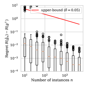
While the bounds hold for any possible distribution \(P\), they are loose for most sensible distributions. Indeed, in many cases, the uniform deviation of the empirical risk \(\sup_{g\in\mathcal{G}} { \lvert R_n(g) - R(g)\rvert }\) over \(\mathcal{G}\) is a very poor bound for \(R(g_n) - R(g^\dagger)\), as mentioned in (Boucheron, Bousquet, and Lugosi 2005 Section 5.2). The looseness of the bound of this section is illustrated in Remark 3..
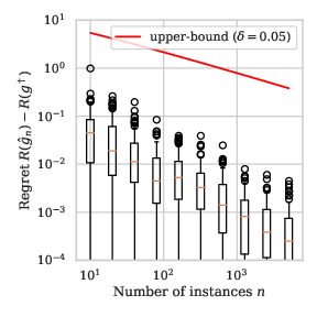
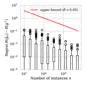
Remark 3: For the distributions defined in Example 1, we illustrate in Section 9 the value of the bound in Proposition 1 for the proposal family of decision stumps in \(\mathbb{R}\).
Firstly, observe that the bound is very loose, which can be explained by the facts that our distribution is not very complicated and our proposal family \(\mathcal{G}_\text{stump}\) is very favorable for the problem at hand.
Secondly, while the order of the slope is the same for any distribution \(P\), the boxplot seems to decrease faster when \(a\) is close to \(1\) than when \(a\) is close to \(0\), i.e. the learning rate for easily separated distributions seems to be faster than \(O(n^{-1/2})\), which is proven in Section 3.
\(a=1/4\)

\(a=1/2\)
\(a=3/4\)
\(a=1/4\)
\(a=1/2\)
\(a=3/4\)
3 - Faster learning bounds
This section introduces the derivations of learning rates faster than \(O(n^{-1/2})\) under a noise assumption on the distribution of the data. Firstly, we introduce concentration inequalities that involve the variance of random variables. Secondly, we introduce noise conditions and explain how they induce an upper-bound on the variance of the excess loss. Finally, we show that combining these two first results gives a fixed-point inequality, which implies fast learning rates.
The methodology presented here is limited to finite classes of functions \(\mathcal{G}\) and to problems for which the Bayes classifier \(g^*\) belongs to \(\mathcal{G}\). In this section, we also discuss the generalization of those results to general classes of functions of controlled complexity that do not contain the Bayes classifier.
We introduce a family of functions \(\mathcal{F}\) such that any \(f\in\mathcal{F}\) corresponds to a \(g \in \mathcal{G}\) with: \[\begin{align} f(X, Y) := \mathbb{I}\{ g(X) \ne Y \} - \mathbb{I}\{ g^*(X) \ne Y \},\end{align}\] i.e. the family \(\mathcal{F}\) is the family of the excess losses of all elements in \(\mathcal{G}\).
The bound of Proposition 1 used the fact that the random variable \(f(X, Y)\) is bounded for any \(g \in \mathcal{G}\). However, in many situations, as we choose a candidate \(g\) that approaches \(g^*\), the variance of \(f(X,Y)\) may be very small in front of the range of \(f(X,Y)\). Since advanced concentrations inequalities exploit the variance of random variables to derive tighter bounds, the next section present concentrations inequalities that use the variance of random variables, which will server to derive tighter bounds than based on hypotheses on the distribution of the data.
3.1 - Advanced concentration inequalities
The derivation of fast learning bounds relies on concentration inequalities that involve the variance of the random variables involved. The simplest one is Bernstein’s inequality, seen in (Boucheron, Lugosi, and Massart 2013 Corollary 2.11). Its proof is featured in (Boucheron, Lugosi, and Massart 2013 Theorem 2.10), and we recall the simplest formulation of the inequality here.
Theorem 1: Let \(Z_1, \dots, Z_n\) be \(n\) i.i.d. real-valued r.v.’s with zero mean, and assume that \({ \lvert Z_i\rvert } \le c\) a.s. Let \(\sigma^2 = \text{Var}(Z_1)\). Then, with \(\bar{Z}_n = (1/n) \sum_{i=1}^n Z_i\), for any \(\delta > 0\), w.p. \(\ge 1-\delta\): \[\begin{align} \bar{Z}_n \le \frac{2c \log(1/\delta)}{3n} + \sqrt{\frac{2\sigma^2 \log(1/\delta)}{n}}. \end{align}\]
Popoviciu’s inequality on variances, see (Egozcue and García 2018), gives an upper bound on the variance of a bounded random variable. Precisely, it states that the variance \(\sigma^2\) of a r.v. \(Z\) such that \(m \le Z \le M\) is smaller than \((M-m)^2/4\). Plugging this result into Theorem 1 gives a similar result as Corollary 3.
Bernstein’s inequality does not give a guarantee on the supremum of a family of functions, but on an empirical mean, as does Hoeffding’s inequality. A direct consequence of Hoeffding’s inequality were guarantees on a finite family of functions, as shown in Corollary 1. As such, only the derivation of guarantees on a finite family of functions are a direct application of the combination of Bernstein’s inequality and noise conditions on \(P\).
To extend those results to more general classes of functions, one requires Talagrand’s inequality below, see (Boucheron, Bousquet, and Lugosi 2005 Section 5.3, Theorem 5.4) for a simple version, and (Boucheron, Lugosi, and Massart 2013 Theorem 7.9, page 225) for the proof. For any \(f \in \mathcal{F}\), we denote by \(Pf := \mathbb{E}[f(X, Y)]\) the distribution of \((X, Y)\) and by \(P_nf := (1/n) \sum_{i=1}^n f(X_i, Y_i)\) the empirical distribution associated to \(\mathcal{D}_n\).
Theorem 3: Let \(b > 0\) and set \(\mathcal{F}\) a family of functions \(\mathcal{X}\to\mathbb{R}\). Assume that, for any \(f \in \mathcal{F}\), \(Pf -f \le b\). Then, w.p \(\ge 1 - \delta\), \[\begin{align} \sup_{f\in\mathcal{F}} (Pf - P_n f) \le 2 \mathbb{E}\left[ \sup_{f\in\mathcal{F}} (Pf - P_nf) \right] + \sqrt{\frac{2 (\sup_{f\in\mathcal{F}} \text{Var}(f) ) \log (1/\delta)}{n} } + \frac{4b \log(1/\delta)}{3n}. \end{align}\]
The formulations of Bernstein’s inequality and Talagrand’s inequality are very similar, and their main difference lies in the fact that, while the first deals with simple means, the second handles the supremum of empirical processes. Note that the first term in the bound of Talagrand’s inequality is controlled in Section 2.2.
These inequalities will prove useful when combined with a clever upper bound of the variance of the excess loss, i.e. the variance of \(f(X,Y)\). Conveniently, that quantity is upper-bounded by a function of the excess risk \(R(g) -R(g^*)\), using the noise conditions introduced in the following section.
3.2 - Noise conditions
The simplest noise assumption to derive faster bounds is called Massart’s noise condition, see (Boucheron, Bousquet, and Lugosi 2005, page 340). It is a local condition on the value of \(\eta\), that assumes that \(\eta(X)\) is always far from \(1/2\), i.e. that there is a clear separation between the two classes for the classification decision.
Assumption 2: There exists \(h > 0\), s.t. \[\begin{align} { \lvert 2\eta(X) - 1\rvert } \ge h \quad \text{a.s.} \end{align}\]
A less restrictive assumption is called the Mammen-Tsybakov noise condition, see (Boucheron, Bousquet, and Lugosi 2005, page 340), and gives a bound on the proportion of \(\mathcal{X}\) for which the classification decision is hard to take. This bound is parameterized by \(a\in[0,1]\). When \(a\) is close to \(1\), it is very easy to separate the two classes, while it is harder when \(a\) is close to \(0\).
Assumption 1: There exists \(B > 0\) and \(a \in [0,1]\), s.t. \[\begin{align} \mathbb{P}\left\{ { \lvert 2\eta(X) - 1\rvert } \le t \right\} \le Bt^{\frac{a}{1-a}}. \end{align}\]
Remark 1: The distribution \((F, \eta)\) introduced in Example 1 satisfies the Mammen-Tsybakov noise condition with parameter \(a\) and \(B=1\).
Observe that Mammen’s noise condition is void when \(a = 0\), and that it is implied with \(a=1\) by Massart’s noise condition. Both noise assumptions can be used to derive a convenient bound on the variance of a function \(f \in \mathcal{F}\), as a consequence of both a second moment bound, i.e. a bound of the form \(\text{Var}(Z) \le \mathbb{E}[Z^2]\), namely: \[\begin{align} \label{eq-var-upper-bound}\tag{12} \text{Var}(f(X,Y)) \le \mathbb{E}[\mathbb{I}\{ g(X) \ne g^*(X) \} ],\end{align}\] and the decomposition of the excess risk presented in Eq. (1): \[\begin{align} R(g) - R(g^*) = \mathbb{E}\left[ { \lvert 2\eta(X)-1\rvert }\mathbb{I}\{g(X) \ne g^*(X) \right].\end{align}\] Combined with Eq. (12) and Eq. (1), Massart’s inequality implies: \[\begin{align} \text{Var}(f(X,Y)) \le \mathbb{E}[\mathbb{I}\{ g(X) \ne g^*(X) \} ] \le \frac{1}{h} \mathbb{E}[ { \lvert 2 \eta(X) - 1\rvert } \mathbb{I}\{ g(X) \ne g^*(X) \} ] = \frac{1}{h}\left( R(g) - R(g^*) \right).\end{align}\] Similarly, the Mammen-Tsybakov noise assumption implies the following proposition.
Proposition 5: Assume that Assumption 1 is true, then, for any \(f \in \mathcal{F}\), there exists \(c\) that depends on only of \(B\) and \(a\), s.t. \[\begin{align} \text{Var}(f(X,Y)) \le c (R(g) - R(g^*))^a \end{align}\]
Proof. The proof relies on Eq. (12) and an equivalent formulation of the Mammen-Tsybakov noise assumption, which states that, there exists \(c > 0\) and \(a \in [0,1]\) such that: \[\begin{align} \mathbb{P}\{ g(X) \ne g^*(X) \} \le c \left( R(g) - R(g^*) \right)^a. \end{align}\] It is implied by Assumption 1. Indeed, Markov’s inequality, i.e. \(\mathbb{I}\{ z > t \} \le z/t\) for any \(z, t \in \mathbb{R}_+\), followed by the Mammen-Tsybakov noise assumption and the observation that \(\mathbb{I}\{A\} \le 1\) for any \(A \in \mathcal{A}\), implies: \[\begin{align} R(g) - R(g^*) &= \mathbb{E}[ { \lvert 2 \eta(X) - 1\rvert } \mathbb{I}\{ g(X) \ne g^*(X) \} ], \\ &\ge t \cdot \mathbb{E}[ \mathbb{I}\{{ \lvert 2 \eta(X) - 1\rvert } > t\} \cdot \mathbb{I}\{ g(X)\ne g^*(X) \} ],\\ &\ge t \cdot \mathbb{P}\{{ \lvert 2 \eta(X) - 1\rvert } > t\} - t \mathbb{E}[ \mathbb{I}\{{ \lvert 2 \eta(X) - 1\rvert } > t\} \cdot \mathbb{I}\{ g(X) = g^*(X) \} ],\\ &\ge (t-Bt^{\frac{1}{1-a}}) - t \mathbb{P}\{ g(X) = g^*(X) \},\\ &\ge t \mathbb{P}\{ g(X) \ne g^*(X) \} - Bt^{\frac{1}{1-a}}. \end{align}\] Taking \(t = \left( \frac{(1-a) \mathbb{P}\{g(X) \ne g^*(X)\}}{B} \right)^{\frac{1-a}{a}}\) gives the result, and \(c = \frac{B^{1-a}}{(1-a)^{1-a} a^a}\). □
Both of the preceding results are contained, or consequences of (Bousquet, Boucheron, and Lugosi 2004 Section 5.2). The proof of Proposition 5 uses an equivalent formulation of Proposition 5, which are proven in (Bousquet, Boucheron, and Lugosi 2004 Definition 7). Those results enable us to derive fast, distribution-dependent generalization bounds, by using those results in conjonction with the concentration inequalities of Section 3.1, and solving a fixed-point equation.
3.3 - Distribution-dependent generalization bounds
The reasoning presented here can be found in (Bousquet, Boucheron, and Lugosi 2004 Section 5.2), but is more detailed here. A union bound of Bernstein’s inequality applied on each element of finite family of \(N\) elements gives that, for any \(\delta > 0\), w.p \(\ge 1-\delta\), we have simultaneously for any \(g \in \mathcal{G}\), with \(f\) the corresponding element in \(\mathcal{F}\): \[\begin{align} \label{eq-bernstein-4-bound}\tag{13} R(g) - R(g^*) \le R_n(g) - R_n(g^*) + \frac{2c \log(N/\delta)}{3n} + \sqrt{\frac{2\text{Var}(f(X,Y)) \log(N/\delta)}{n}}.\end{align}\] Combining Eq. (13) with the implications of the Mammen-Tsybakov noise assumption, i.e. with Proposition 5, for the empirical risk minimizer and under the assumption that \(g^*\) belongs to the proposal class, i.e. for \(g = g_n\) and that \(g^* \in \mathcal{G}\), we have: for any \(\delta > 0\), w.p \(\ge 1-\delta\), \[\begin{align} \label{eq-fixed-point-4-bound}\tag{14} R(g_n) - R(g^*) \le \frac{2c \log(N/\delta)}{3n} + (R(g_n) - R(g^*))^{a/2} \sqrt{\frac{2c \log(N/\delta)}{n}},\end{align}\] which is a fixed point inequality in \(R(g_n) - R(g^*)\). To derive an upper-bound on \(R(g_n) - R(g^*)\) from Eq. (14), we use the following Lemma, which is found in (Cucker and Smale 2002 Lemma 7).
Lemma 2: Let \(c_1, c_2 > 0\) and \(s > q > 0\). Then the equation \(x^s - c_1 x^q - c_2 = 0\) has a unique positive zero \(x^*\). In addition, \(x^* \le \max \{ (2c_1)^{1/(s-q)}, (2c_2)^{1/s} \}\).
Proof. Define \(\varphi(x) = x^s - c_1 x^q - c_2\). Then \(\varphi'(x) = x^{q-1}(s x^{s-q} - q c_1 )\). Thus \(\varphi'(x) = 0\) with \(x > 0\) if and only if \(x^{s-q} = qc_1/s\) which proves that \(\varphi'(x)\) has a unique positive zero. Since \(\varphi(x) < 0\), \(\lim_{x \overset{>}{\to} 0} \varphi'(x) \le 0\) and \(\lim_{x\to\infty} \varphi(x) = +\infty\), then \(\varphi(x)\) has a unique positive zero.
A generalization of Theorem 4.2 of (Mignotte 1992), which gives an upper bound on the maximum of the absolute values of the roots of a polynomial, implies the result. □
Using Lemma 2, we can prove a fast learning bound for finite families of functions.
Proposition 4: Assume that \(\mathcal{G}\) is a finite family of \(N\) functions and that the Mammen-Tsybakov noise assumption is verified with noise parameter \(a\). For any \(\delta > 0\), we have that, w.p. \(\ge 1-\delta\), \[\begin{align} R(g_n) - R(g^*) &\le \left ( \frac{8 c\log (N/\delta) }{ n} \right )^{1/(2-a)} + \frac{8 c \log (N / \delta) }{ 3n }. \end{align}\]
Proof. The straightforward application of Lemma 2 to Eq. (14), followed by the bound \(\max(x, y) \le x + y\) for \(x,y > 0\) implies: \[\begin{align} R(g_n) - R(g^*) &\le \max \left ( \left ( \frac{8 c\log (N/\delta) }{ n} \right )^{1/(2-a)}, \frac{8 c \log (N / \delta) }{ 3n } \right ),\\ &\le \left ( \frac{8 c\log (N/\delta) }{ n} \right )^{1/(2-a)} + \frac{8 c \log (N / \delta) }{ 3n }. \end{align}\] □
Proposition 4 gives a learning bound of the order \(O(n^{-\frac{1}{2-a}})\), under a noise condition parameterized by \(a \in [0,1]\). When \(a\) is close to \(0\), one recovers the order \(O(n^{-\frac{1}{2}})\) derived in Section 2.3. On the other hand, when \(a\) is close to zero, one approaches the fast rate \(O(n^{-1})\). The fast bounds are illustrated in Remark 3. The generalization of Proposition 4 to non-finite families of functions is more involved and is a consequence of Talagrand’s inequality (Theorem 3), and we refer to (Boucheron, Bousquet, and Lugosi 2005 Section 5.3) for that extension. The analysis presented there extends to the case where \(g^*\) does not belongs to \(\mathcal{G}\), which is detailed in (Boucheron, Bousquet, and Lugosi 2005 Section 5.3.5).
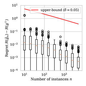
Remark 2: With the distributions defined in Example 1, we illustrate the value of the bound in Proposition 4 for the finite proposal family of functions \(\mathcal{G} = \{ i/100 \mid i\in \{ 0, \dots, 1\}\) in Section 9.
Observe in Section 12 that the learning rate of the fast bound seems much more aligned with the empirical learning rate than the one of Section 2.
\(a=1/4\)
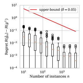
\(a=1/2\)
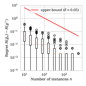
\(a=3/4\)
In real problems, as the distribution of the data is unknown, one can not verify whether a noise assumption is satisfied by the distribution of the data. Still, fast learning speeds partially justify the looseness of the bounds derived in Section 2 and constitute strong evidence of the soundness of learning from empirical data.
Bibliography
Boucheron, Stéphane, Olivier Bousquet, and Gàbor Lugosi. 2005. “Theory of Classification : A Survey of Some Recent Advances.” ESAIM: Probability and Statistics 9: 323–75.
Boucheron, Stéphane, Gábor Lugosi, and Pascal Massart. 2013. Concentration Inequalities: A Nonasymptotic Theory of Independence. OUP Oxford.
Bousquet, Olivier, Stéphane Boucheron, and Gàbor Lugosi. 2004. “Introduction to Statistical Learning Theory.” In Advanced Lectures on Machine Learning, 169–207.
Cucker, Felipe, and Steve Smale. 2002. “Best Choices for Regularization Parameters in Learning Theory: On the Bias-Variance Problem.” Foundations of Computational Mathematics 2 (January): 413–28.
Domingos, Pedro. 2012. “A Few Useful Things to Know About Machine Learning.” Commun. ACM 55 (10): 78–87. https://doi.org/10.1145/2347736.2347755.
Egozcue, Martín, and Luis Fuentes García. 2018. “The Variance Upper Bound for a Mixed Random Variable.” Communications in Statistics - Theory and Methods 47 (22): 5391–9395. https://doi.org/10.1080/03610926.2017.1390136.
Györfi, László. 2002. Principles of Nonparametric Learning. Edited by László Györfi. Springer. https://doi.org/10.1017/CBO9781107415324.004.
Jost, Jürgen. 2011. Riemannian Geometry and Geometric Analysis. https://doi.org/10.1007/978-3-642-21298-7.
Mignotte, Maurice. 1992. Mathematics for Computer Algebra. Berlin, Heidelberg: Springer-Verlag.
Mohri, Mehryar, Afshin Rostamizadeh, and Ameet Talwalkar. 2012. Foundations of Machine Learning. MIT Press. http://www.jstor.org/stable/j.ctt5hhcw1.
Papoulis, A. 1965. Probability, Random Variables, and Stochastic Processes. McGraw-Hill.
Shalev-Shwartz, Shai, and Shai Ben-David. 2014. Understanding Machine Learning: From Theory to Algorithms. USA: Cambridge University Press.
Shorack, Galen. 2000. “Probability for Statisticians.” Springer. https://doi.org/10.1198/jasa.2002.s481.
Smale, Steve, and Ding-Xuan Zhou. 2011. “Estimating the Approximation Error in Learning Theory.” Analysis and Applications 01 (November). https://doi.org/10.1142/S0219530503000089.
Back to article list - Written on the 20/03/20.